Python Quantitative Trading

Python quantitative trading refers to the process of using the Python programming language along with related libraries and tools to analyze financial market data, develop strategies, and execute trades.

Python has become one of the preferred programming languages for quantitative trading due to its simplicity, ease of learning, powerful ecosystem, and rich financial libraries.

Quantitative trading is widely used in the financial field, allowing traders to formulate and execute trading strategies through systematic methods, improving trading efficiency and the scientific nature of decision-making.

Quantitative trading mainly involves using mathematical and statistical methods to perform quantitative analysis of financial markets through computer technology, thereby formulating and executing trading strategies.

For more Python quantitative trading content, see: Python Quantitative Trading.

---

Example Application

Let’s first look at a simple Python quantitative trading example using a moving average strategy with Yahoo Finance data.

The basic idea of this strategy is to generate buy and sell signals by comparing short-term and long-term moving averages.

Before running this simple example, you need to install three packages:

pip install pandas yfinance matplotlib

Package Description:

• Pandas is a powerful open-source data processing and analysis library, specifically designed for efficient data analysis and manipulation.
• yfinance is a library for fetching financial data, supporting the retrieval of stocks, indices, and other financial market data from Yahoo Finance.
• Matplotlib is a 2D plotting library for creating static, dynamic, and interactive data visualization charts.

Fetching Historical Stock Data

Use yfinance to fetch historical stock data. Here is a simple example:

Example

import yfinance as yf

# Fetch stock data
symbol = "600519.SS"
start_date = "2022-01-01"
end_date = "2023-01-01"

data = yf.download(symbol, start=start_date, end=end_date)
print(data.head())

Output result is as follows:

                  Open         High          Low        Close    Adj Close   Volume
Date                                                                               
2022-01-04  2055.00000  2068.949951  2014.000000  2051.229980  1973.508057  3384262
2022-01-05  2045.00000  2065.000000  2018.000000  2024.000000  1947.309937  2839551
2022-01-06  2022.01001  2036.000000  1938.510010  1982.219971  1907.112915  5179475
2022-01-07  1975.00000  1988.880005  1939.319946  1942.000000  1868.416870  2981669
2022-01-10  1928.01001  1977.000000  1917.550049  1966.000000  1891.507446  2962670

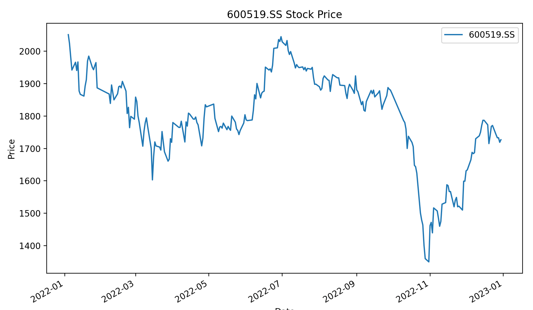
Simple Data Analysis and Visualization

Use pandas for data analysis and matplotlib for visualization:

Example

import yfinance as yf
import pandas as pd
import matplotlib.pyplot as plt

# Fetch stock data
symbol = "600519.SS"
start_date = "2022-01-01"
end_date = "2023-01-01"

data = yf.download(symbol, start=start_date, end=end_date)
# Simple data analysis
print(data.describe())

# Plot stock price trend
data['Close'].plot(figsize=(10, 6), label=symbol)
plt.title(f"{symbol} Stock Price")
plt.xlabel("Date")
plt.ylabel("Price")
plt.legend()
plt.show()

The trend chart is displayed as follows:

Moving Average Crossover Strategy Backtest

Backtesting is the process of simulating and evaluating a trading strategy on historical market data.

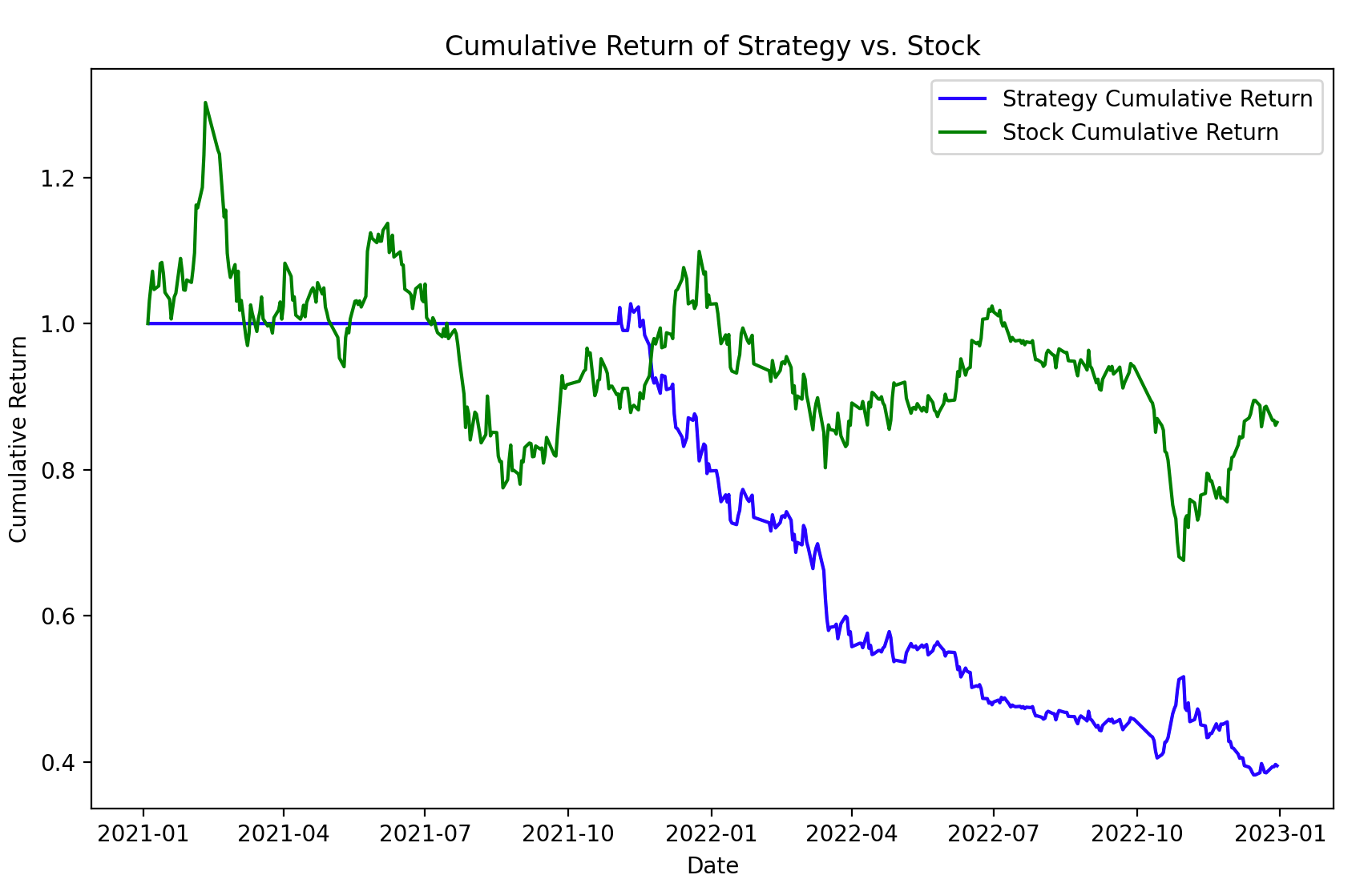
The following is an example code for a simple moving average crossover strategy backtest. The strategy buys when the 50-day moving average crosses above the 200-day moving average, and sells when it crosses below. The strategy’s performance is output with indicators such as total return, annualized return, and maximum drawdown.

Example

import yfinance as yf
import pandas as pd
import matplotlib.pyplot as plt

# Fetch stock data
symbol = "600519.SS"
start_date = "2021-01-01"
end_date = "2023-01-01"

data = yf.download(symbol, start=start_date, end=end_date)

# Calculate moving averages
data['SMA_50'] = data['Close'].rolling(window=50).mean()
data['SMA_200'] = data['Close'].rolling(window=200).mean()

# Initialize signal column
data['Signal'] = 0

# Calculate crossover signals
data.loc[data['SMA_50'] > data['SMA_200'], 'Signal'] = 1
data.loc[data['SMA_50'] < data['SMA_200'], 'Signal'] = -1

# Calculate daily returns
data['Daily_Return'] = data['Close'].pct_change()

# Calculate strategy signal returns (shift(1) is to avoid look-ahead bias)
data['Strategy_Return'] = data['Signal'].shift(1) * data['Daily_Return']

# Calculate cumulative returns
data['Cumulative_Return'] = (1 + data['Strategy_Return']).cumprod()

# Output strategy performance
strategy_performance = {
    'Total Return': data['Cumulative_Return'].iloc[-1] - 1,
    'Annualized Return': (data['Cumulative_Return'].iloc[-1] ** (252 / len(data))) - 1,
    'Max Drawdown': (data['Cumulative_Return'] / data['Cumulative_Return'].cummax() - 1).min(),
}

print("Strategy Performance:")
for key, value in strategy_performance.items():
    print(f"{key}: {value:.4f}")

# Plot cumulative return curve
plt.figure(figsize=(10, 6))
plt.plot(data['Cumulative_Return'], label='Strategy Cumulative Return', color='b')
plt.plot(data['Close'] / data['Close'].iloc[0], label='Stock Cumulative Return', color='g')
plt.title("Cumulative Return of Strategy vs. Stock")
plt.xlabel("Date")
plt.ylabel("Cumulative Return")
plt.legend()
plt.show()

The display chart is as follows:

Please note that this is just a simple example. In practical applications, more complex strategies and more considerations are needed.